vaspparser demo

This notebook walks through the main building blocks of the vaspparser package using the sample VASP output files that ship with the test suite (tests/static/vasp_test_files).

It covers:

1. Reading and writing VASP structure files (POSCAR/CONTCAR)

2. Parsing a full VASP run with parse_vasp_output

3. Parsing individual files: OSZICAR, OUTCAR, vasprun.xml, PROCAR

4. Working with the electronic structure: density of states (DOS) and the band gap

5. Reading volumetric data (CHGCAR)

6. Bader charge analysis helpers

import os

import numpy as np

# Sample VASP output files used throughout the test suite
TEST_FILES = os.path.join("static", "vasp_test_files")
FULL_JOB_SAMPLE = os.path.join(TEST_FILES, "full_job_sample")

1. Reading and writing structures

VASP structures are stored in the POSCAR/CONTCAR format. read_atoms parses such a file into an ASE Atoms object, and write_poscar does the reverse.

from vaspparser.vasp.structure import read_atoms, write_poscar, vasp_sorter

structure = read_atoms(os.path.join(FULL_JOB_SAMPLE, "POSCAR"), species_list=["Fe"])
structure

Atoms(symbols='Fe2', pbc=True, cell=[2.8, 2.8, 2.8])

# vasp_sorter() gives the permutation that groups atoms by species, which is how VASP
# expects atoms to be ordered inside a POSCAR file
vasp_sorter(structure)

array([0, 1])

write_poscar(structure=structure, filename="POSCAR_demo")
roundtrip = read_atoms("POSCAR_demo")
assert roundtrip == structure
os.remove("POSCAR_demo")
roundtrip

Atoms(symbols='Fe2', pbc=True, cell=[2.8, 2.8, 2.8])

2. Parsing a full VASP run

parse_vasp_output is the main entry point of the package: point it at a calculation directory and it returns a single, hierarchical dictionary with everything that could be parsed (energies, forces, structure, electronic structure, charge density, …).

from vaspparser.vasp.output import parse_vasp_output

output_dict = parse_vasp_output(working_directory=FULL_JOB_SAMPLE)
list(output_dict.keys())

['description',
 'generic',
 'structure',
 'charge_density',
 'electronic_structure',
 'outcar']

# Generic, code-agnostic quantities (energies, forces, positions, ...)
list(output_dict["generic"].keys())

['temperature',
 'stresses',
 'pressures',
 'elastic_constants',
 'forces',
 'cells',
 'volume',
 'energy_pot',
 'energy_tot',
 'steps',
 'positions',
 'dft']

energy_tot = output_dict["generic"]["energy_tot"]
print(f"Number of ionic steps: {len(energy_tot)}")
print(f"Final total energy: {energy_tot[-1]:.6f} eV")

Number of ionic steps: 1
Final total energy: -17.737987 eV

3. Parsing individual output files

Each VASP file also has a dedicated parser that can be used on its own.

OSZICAR

The OSZICAR file tracks the energy at every electronic/ionic step.

from vaspparser.vasp.parser.oszicar import Oszicar

oszicar = Oszicar()
oszicar.from_file(filename=os.path.join(FULL_JOB_SAMPLE, "OSZICAR"))
oszicar.parse_dict["energy_pot"]

array([-17.73798679])

OUTCAR

The OUTCAR file contains most of what VASP printed during the run: energies, forces, stresses, the Fermi level, magnetic moments, and more.

from vaspparser.vasp.parser.outcar import Outcar

outcar = Outcar()
outcar.from_file(filename=os.path.join(FULL_JOB_SAMPLE, "OUTCAR"))
print("Fermi level (eV):", outcar.parse_dict["fermi_level"])
print("Number of electrons:", outcar.parse_dict["n_elect"])
print("Final pressure:", outcar.parse_dict["pressures"][-1])

Fermi level (eV): 5.9788
Number of electrons: 16.0
Final pressure: [-0.08177043 -0.08177043 -0.08177043]

vasprun.xml

vasprun.xml is VASP’s structured XML output and is the preferred source for energies, forces, and the electronic structure when available.

from vaspparser.vasp.vasprun import Vasprun

vasprun_path = os.path.join(TEST_FILES, "vasprun_samples", "vasprun_2.xml")
vasprun = Vasprun()
vasprun.from_file(filename=vasprun_path)
print("Final energy (eV):", vasprun.vasprun_dict["total_fr_energies"][-1])

Final energy (eV): -67.64570454

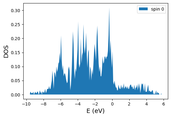
4. Electronic structure: DOS and band gap

Vasprun.get_electronic_structure() returns an ElectronicStructure object with the eigenvalues/occupancies for every k-point and spin channel. From there we can compute the density of states and the band gap.

electronic_structure = vasprun.get_electronic_structure()
print("Eigenvalue matrix shape (spin, kpoints, bands):", electronic_structure.eigenvalue_matrix.shape)
electronic_structure.get_band_gap()

Eigenvalue matrix shape (spin, kpoints, bands): (1, 36, 72)

{0: {'band_gap': np.float64(0.007800000000000001),
  'vbm': {'value': np.float64(-0.1611),
   'kpoint': <vaspparser.dft.waves.electronic.Kpoint at 0x7544a5a8b4d0>,
   'band': <vaspparser.dft.waves.electronic.Band at 0x7544a594fb30>},
  'cbm': {'value': np.float64(-0.1533),
   'kpoint': <vaspparser.dft.waves.electronic.Kpoint at 0x7544a5a8b1c0>,
   'band': <vaspparser.dft.waves.electronic.Band at 0x7544a5908230>}}}

from vaspparser.dft.waves.dos import Dos

dos = Dos(es_obj=electronic_structure, n_bins=200)
plot = dos.plot_total_dos()
plot.show()

PROCAR

The PROCAR file holds atom- and orbital-projected band/DOS information, useful for analysing the chemical character of bands.

from vaspparser.vasp.procar import Procar

procar = Procar()
procar_es = procar.from_file(filename=os.path.join(TEST_FILES, "PROCAR_for_test"))
band = procar_es.kpoints[0].bands[0][0]
print("Eigenvalue:", band.eigenvalue, "Occupancy:", band.occupancy)
print("Per-atom resolved DOS:", band.atom_resolved_dos)

Eigenvalue: -17.37867948 Occupancy: 1.0
Per-atom resolved DOS: [0.145 0.298 0.298]

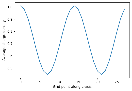
5. Volumetric data: charge density

CHGCAR/LOCPOT-style files describe a quantity on a real-space grid. VaspVolumetricData parses them and offers helpers such as averaging the density along one lattice direction (handy for e.g. work-function or interface analysis).

from vaspparser.vasp.volumetric_data import VaspVolumetricData

charge_density = VaspVolumetricData()
charge_density.from_file(filename=os.path.join(FULL_JOB_SAMPLE, "CHGCAR"), normalize=True)
print("Grid shape:", charge_density.total_data.shape)

average_along_c = charge_density.get_average_along_axis(ind=2)
average_along_c

Grid shape: (28, 28, 28)

array([1.00830804, 0.98088211, 0.90377918, 0.79195173, 0.66754708,
       0.55462055, 0.47555225, 0.44711719, 0.47555225, 0.55462055,
       0.66754708, 0.79195173, 0.90377918, 0.98088211, 1.00830804,
       0.98088211, 0.90377918, 0.79195173, 0.66754708, 0.55462055,
       0.47555225, 0.44711719, 0.47555225, 0.55462055, 0.66754708,
       0.79195173, 0.90377918, 0.98088211])

import matplotlib.pyplot as plt

plt.figure(figsize=(6, 4))
plt.plot(average_along_c)
plt.xlabel("Grid point along c-axis")
plt.ylabel("Average charge density")
plt.show()

6. Bader charge analysis

Bader analysis partitions the charge density into atomic basins. Running the actual analysis requires the external bader executable, but vaspparser also exposes helpers to parse its output (ACF.dat) and to combine AECCAR0/AECCAR2 into the valence and total charge density used as the Bader input.

from vaspparser.dft.bader import parse_charge_vol_file, get_valence_and_total_charge_density

bader_test_path = os.path.join(TEST_FILES, "bader_test")
bader_structure = read_atoms(os.path.join(bader_test_path, "POSCAR"))

acf_file = os.path.join("static", "dft", "bader_files", "ACF.dat")
charges, volumes = parse_charge_vol_file(structure=bader_structure, filename=acf_file)
print("Bader charges:", charges)
print("Bader volumes:", volumes)

Bader charges: [0.438202 0.438197 7.143794]
Bader volumes: [287.28469  297.577878 415.155432]

charge_density_valence, charge_density_total = get_valence_and_total_charge_density(
    working_directory=bader_test_path
)
print("Valence charge density grid:", charge_density_valence.total_data.shape)
print("Total (core + valence) charge density grid:", charge_density_total.total_data.shape)

Valence charge density grid: (20, 20, 20)
Total (core + valence) charge density grid: (20, 20, 20)